Overview
IncSFA extracts slow features without storing or estimating computationally expensive covariance matrices of the input data. This makes it suitable to use IncSFA for applications with high-dimensional images as inputs. However, if the statistics of the inputs change over time, like most online-learning approaches, IncSFA gradually forgets previously learned representations, Curiosity-Driven Modular Incremental Slow Feature Analysis (Curious Dr. MISFA) uses the theory of artificial curiosity to address the forgetting problem faced by IncSFA, by retaining what was previously learned in the form of expert modules. From a set of input video streams, Curious Dr. MISFA actively learns multiple expert modules comprising slow feature abstractions in the order of increasing learning difficulty, with theoretical guarantees.
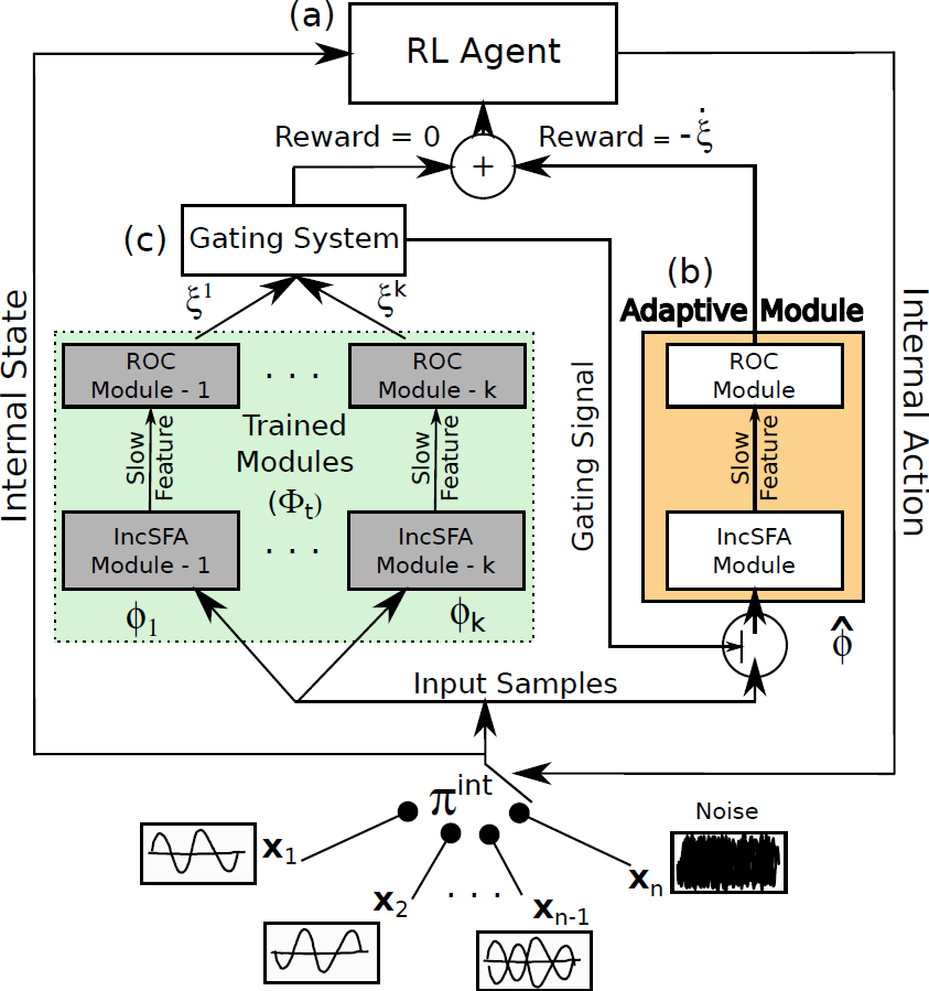
Figure 4 shows the architecture of Curious Dr. MISFA.
- Input: A set of pre-defined high-dimensional observation streams $X = \{{\bf x_1}, ..., {\bf x_n}: {\bf x_i}(t) \in \mathbb{R}^{I}, I \in \mathbb{N}\}$.
- RL agent: An rl agent is in an internal environment with a state-space: $ \mathcal{S}^{\text{int}} = \{s^{\text{int}}_1,...,s^{\text{int}}_n\}$, equal to the number of observation streams. At each state the agent can take two internal actions: $\mathcal{A}^{\text{int}} = \{\text{stay}, \text{switch}\}$. The action stay makes the agent's internal state to be the same as the previous state, while switch randomly shifts the agent's state to one of the other internal states. The agent at each state $s^{\text{int}}_i$ receives a fixed $\tau$ time step sequence of observations (${\bf x}$) of the corresponding stream ${\bf x}_i$.
- Adaptive IncSFA-ROC module An adaptive IncSFA is coupled with a Robust Online Clustering (ROC) algorithm to learn an abstraction $\widehat{\phi}$ based on the incoming observations. $\xi$ denotes the estimation-error made by the IncSFA-ROC for the input-samples ${\bf x}$.
- Gating system The gating system contains previously learned frozen abstractions $\{ \phi_1, ..., \phi_k\}$. It prevents encoding new observations that have been previously encoded.
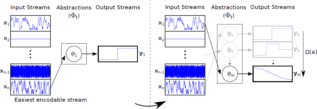
- Goal The desired result of Curious Dr. MISFA is a sequence of abstractions $\Phi_t = \{\phi_1,...,\phi_m; m \le n\}$ learned in the order of increasing learning difficulty. Each abstraction $\phi_i: {\bf x} \rightarrow {\bf y}$ is unique and maps one or more observation streams ${\bf x} \in X$ to a low-dimensional output ${\bf y}(t) \in \mathbb{R}^J, J \in \mathbb{N}$. However, since the learning difficulty of the observation streams is not known a priori, the learning process involves estimating not just the abstractions, but also the order in which the observation streams are encoded. To this end, Curious Dr. MISFA uses the internal RL agent to learn an optimal observation stream selection policy $\pi^{\text{int}}: \mathcal{S}^{\text{int}} \rightarrow \mathcal{A}^{\text{int}}$ that optimizes the following cost-function: $$ \mathcal{J} = \min_{\pi^{\text{int}}} ~ (\langle\dot{\xi}\rangle_t^{\tau}, \langle\xi\rangle_t^{\tau}).$$ The above equation is a Multi-Objective Reinforcement Learning problem, where $\langle\dot{\xi}\rangle_t^{\tau}$ is time-derivative of the $\tau$-window averaged error $\langle\xi\rangle_t^{\tau}$. Minimization of the first objective would result in a policy that will shift the agent to states where the error decreases sharply ($\langle\dot{\xi}\rangle_t^{\tau} < 0 $), indicating faster learning progress of the abstraction-estimator. Minimization of the second objective results in a policy that improves the developing abstraction to better encode the observations. The two objectives are correlated but partially conflicting. I use an approach to find a dynamically changing pareto-optimal policy, by prioritizing each objective based on the error $\xi$. To this end, the cost is scalarized in terms of a scalar reward $r^{\text{int}}$ that evaluates the input ${\bf x}$ received for the tuple $(s^{\text{int}},a^{\text{int}},s^{\text{int}}_{-})$ as follows: $$ r^{\text{int}} = \left(\alpha\langle\dot{\xi}\rangle_t^{\tau} + \beta Z(|\delta- \langle\xi\rangle_t^{\tau}|)\right),$$ where $Z$ is a normally distributed random variable with mean $\delta$ and standard deviation $\sigma$. Here, $\alpha,~\beta,~\delta$ and $\sigma$ are constant scalars.
- Exploration-Exploitation Tradeoff To balance between exploration and exploitation, a decaying $\epsilon$-greedy strategy over the policy $\pi^{\text{int}}$ is used to carry out an action (stay or switch) for the next iteration. When the $\epsilon$ value decays to zero, the agent exploits the policy and an abstraction is learned.
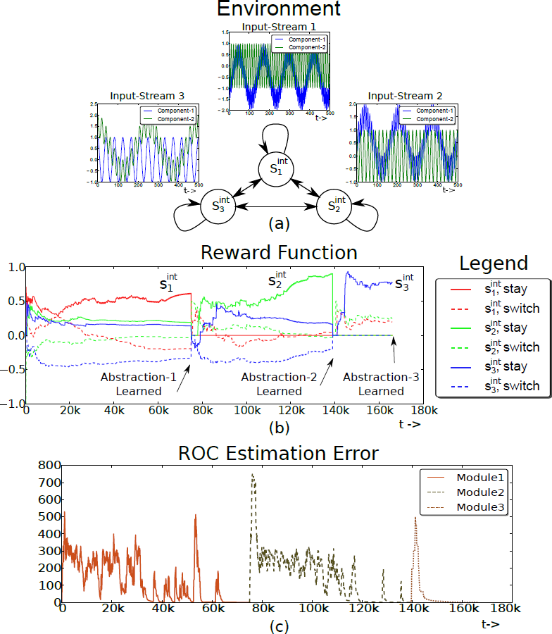
Figure 6 shows a simple proof-of-concept experimental result conducted using three 2D oscillatory audio streams.
The environment has three internal states $\mathcal{S}^{\text{int}} = \{s^{\text{int}}_1, s^{\text{int}}_2, s^{\text{int}}_3\}$ associated with the
observation streams (Figure 6(a)). The stream ${\bf x}_1$ is the easiest signal to
encode followed by the input streams ${\bf x}_2$ and ${\bf x}_3$. The dynamics of the algorithm can be observed by studying
the time varying reward function $R^{\text{int}}$ and the ROC estimation error $\xi$.
Figure 6(b) shows the reward function for a single run of the
experiment. Solid lines represent the reward for the action
stay in each state $s^{\text{int}}_i$, while the dotted
lines represent the marginalized reward for the action switch at
each state. For the sake of explanation, the learning process can be thought of as passing through three phases, where
each phase corresponds to learning a single abstraction module.
Phase 1: At the beginning of Phase 1, the agent starts exploring by
executing either stay or switch at each state. After a few hundred
algorithm iterations, the reward function begins to stabilize and is such that
$R^{\text{int}}(s^{\text{int}}_1,$ stay$) > R^{\text{int}}(s^{\text{int}}_2,$ stay$) > R^{\text{int}}(s^{\text{int}}_3,$ stay$) > 0$,
ordered according to the learning difficulty of the observation streams. However, the
reward components for the switch action are either close to zero or
negative. Therefore, the policy $\pi^{\text{int}}$ converges to the
optimal policy (i.e. to stay at the state corresponding to the
easiest observation stream ${\bf x}_1$ and switch at every other state). As $\epsilon$
decays, the agent begins to exploit the learned policy, and the adaptive
IncSFA-ROC abstraction $\widehat{\phi}$ converges to the slow feature
corresponding to the observation stream ${\bf x}_1$. The ROC estimation error (Figure
6(c)) decreases and falls below the threshold $\delta$, at
which point, the abstraction is added to the abstraction set $\Phi$. The
increase in the reward value of $R^{\text{int}}(s^{\text{int}}_1,$ stay$)$ near the end of the
phase is caused by the second term ($\sum_{\tau}\left(Z(|\delta - \xi^{roc}|\right)$) in the reward equation. Both
$\epsilon$ and $R^{\text{int}}$ are reset and the algorithm enters Phase 2 at ($t \approx
75k$).
Phase 2: The agent begins to explore again, however, it does not receive
any reward for the ($s^{\text{int}}_1$, stay) tuple because of the gating system.
After a few hundred algorithm iterations, $R^{\text{int}}(s^{\text{int}}_2,$ stay$) > R^{\text{int}}(s^{\text{int}}_3,$
stay$) > R^{\text{int}}(s^{\text{int}}_1,$ stay$)=0$, the
adaptive abstraction converges, but to the slow feature corresponding to the
observation stream ${\bf x}_2$.
Phase 3: The process continues again until the third abstraction is learned. A link to the Python implementation
of the Curious Dr. MISFA algorithm can be found in the Software section
below.
Videos
Software
Python (requires PyQtGraph)