Overview
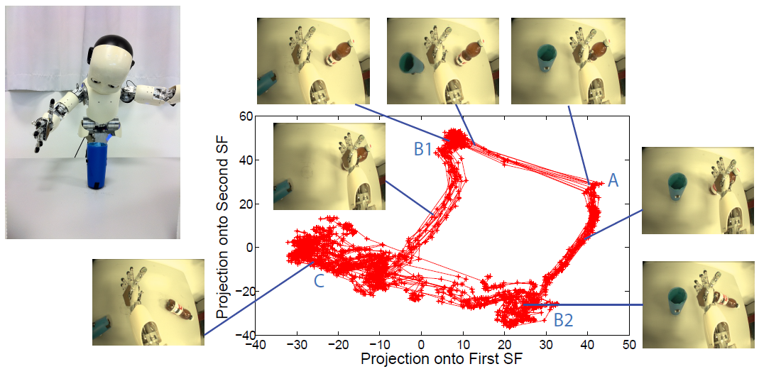
Slow Feature Analysis (SFA) is an unsupervised learning algorithm that extracts instantaneous features of slowly varying components within a fast varying input signal. Similar to the well known Principal Component Analysis (PCA) algorithm, SFA is linear and has a closed form solution. But unlike the PCA, the extracted features explain the directions of the slowest variations in the input. These slowest variations usually correspond to the underlying causes of the changing sensory inputs. When applied to a sequence of high-dimensional image observations captured by an exploring agent, SFA extracts invariant features encoding the agent's pose, making it potentially useful for vision based path planning.
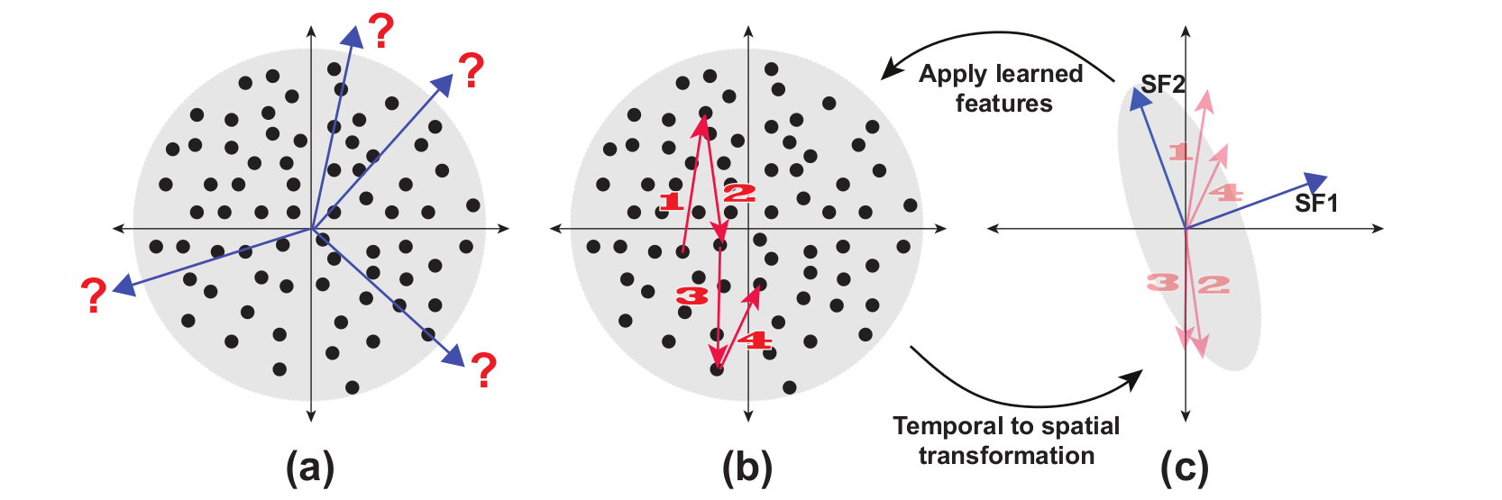
Incremental Slow Feature Analysis (IncSFA) is a low complexity, unsupervised learning technique that updates slow features incrementally. IncSFA follows the learning objective of the batch SFA (BSFA), which is as follows: given an I-dimensional sequential input signal ${\bf x}(t) = [x_{1}(t), ..., x_{I}(t)]^{T},$ find a set of $J$ instantaneous real-valued functions ${\bf g}(x) = [g_{1}({\bf x}), ...,g_{J}({\bf x})]^{T},$ which together generate a $J$-dimensional output signal ${\bf y}(t) = [y_{1}(t), ...,y_{J}(t)]^{T}$ with $y_{j}(t) = g_{j}({\bf x}(t))$, such that for each $j \in \{1, ...,J\}$ $$ \Delta_{j} = \Delta(y_{j}) = \langle\dot{y}_{j}^{2}\rangle \quad \text{is minimal} $$ under the constraints $$ \langle y_{j} \rangle = 0\quad\textrm{(zero mean),}$$ $$ \langle y_{j}^{2} \rangle = 1\quad\textrm{(unit variance),} $$ $$ \forall i < j: \langle y_{i}y_{j} \rangle = 0\quad\textrm{(decorrelation and order),}$$ where $\langle \cdot \rangle$ and $\dot{y}$ indicates temporal averaging and the derivative of $y$, respectively. The problem is to find instantaneous functions $g_j$ that generate different output signals varying as slowly as possible. These functions are called slow features. See Figure 1 for a visual example of the meaning of a slow feature. The constraints together avoid a trivial constant output solution. The decorrelation constraint ensures that different functions $g_j$ do not code for the same features.
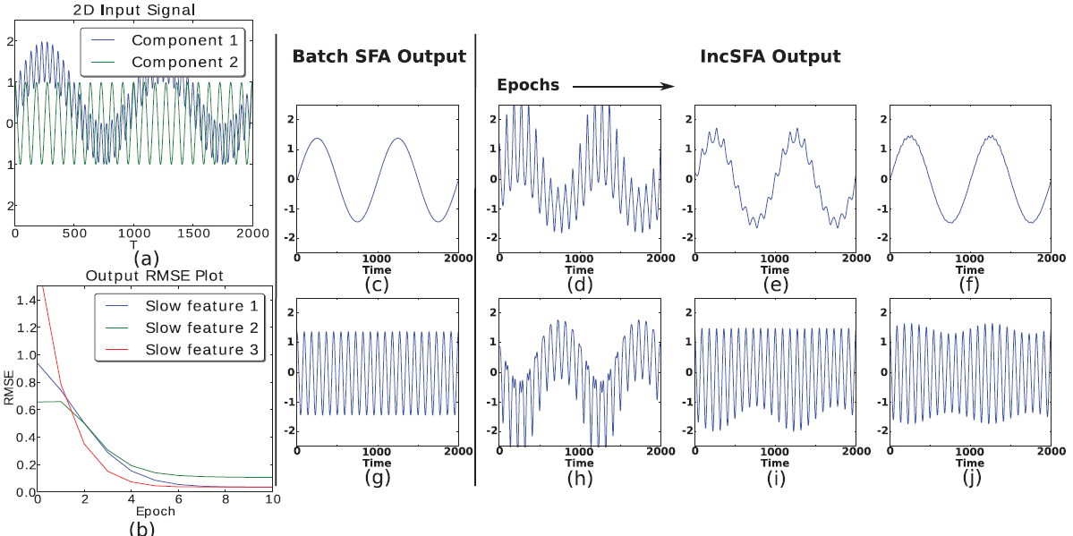
BSFA solves a linear approximation of the above problem through a simpler eigenvector approach. It applies batch Principle Component Analysis (PCA) twice. The first PCA is used to normalize the input ${\bf x}$ to have a zero mean and identity covariance matrix (whitening). The second PCA is applied on the derivative of the normalized input $\dot{{\bf z}}$. The eigenvectors with the least eigenvalues are the slow feature vectors.
IncSFA replaces the batch PCA algorithms with their incremental alternatives. To replace the first PCA, IncSFA uses the state-of-the-art Candid Covariance-Free Incremental PCA (CCIPCA). CCIPCA incrementally whitens the date without keeping an estimate of the covariance matrix. Except for the low-dimensional derivative signals $\dot{{\bf z}}$, CCIPCA cannot replace the second PCA step. It takes a long time to converge to the slow features, since they correspond to the least significant components. Minor Components Analysis (MCA) incrementally extracts principal components, but with a reversed preference: it extracts the components with the smallest eigenvalues fastest. IncSFA uses a modified version of Peng's low complexity MCA updating rule, and Chen's Sequential Addition technique to extract multiple slow features in parallel. A high-level formulation of IncSFA is $$(\phi(t+1), {\bf V}(t+1)) = IncSFA\left(\phi(t), {\bf V}(t), {\bf x}(t), \theta(t)\right),$$ where $\phi(t) = \left(\phi_1(t), ...,\phi_J(t)\right)$ is the matrix of existing slow feature vector estimates for $J$ slow features and ${\bf V} = \left({\bf v}_1, ..., {\bf v}_K \right)$ is the matrix of $K$ principal component vector estimates used to construct the whitening matrix. Here ${\bf x}(t) \in \mathbb{R}^I, I \in \mathbb{N}$ is the input observation and $\theta$ contains parameters about setting learning rates.
For many instances, there is no need to use IncSFA instead of BSFA. But at higher dimensionality, IncSFA becomes more and more appealing. For some problems with very high dimensionality and limited memory, IncSFA could be the only option, e.g., an autonomous robot with limited onboard hardware, which could still learn slow features from its visual stream via IncSFA. The following summarizes the advantages IncSFA has over BSFA:
- it is adaptive to changing input statistics;
- it has linear computational efficiency as opposed to cubic of BSFA;
- it has reduced sensitivity to outliers;
- it adds to the biological plausibility of BSFA.
These advantages make IncSFA suitable to use for several online learning applications. A link to the Python, Matlab, javascript (browser) implementation of the IncSFA algorithm can be found in the Software section below.