Slowness Learning for Curiosity-Driven Agents

Abstract

In the absence of external guidance, how can a baby humanoid robot learn to map the many raw pixels of high-dimensional visual inputs to useful action sequences? I study methods that achieve this by making robots self-motivated (curious) to continually build compact representations of sensory inputs that encode different aspects of the changing environment. Previous curiosity-based agents acquired skills by associating intrinsic rewards with world model improvements, and used reinforcement learning (RL) to learn how to get these intrinsic rewards. But unlike in previous implementations, I consider streams of high-dimensional visual inputs, where the world model is a set of compact low-dimensional representations of the high-dimensional inputs. To learn these representations, I use the slowness learning principle, which states that the underlying causes of the changing sensory inputs vary on a much slower time scale than the observed sensory inputs. The representations learned through the slowness learning principle are called slow features (SFs). Slow features have been shown to be useful for RL, since they capture the underlying transition process by extracting spatio-temporal regularities in the raw sensory inputs. However, existing techniques that learn slow features are not readily applicable to curiosity-driven online learning agents, as they estimate computationally expensive covariance matrices from the data via batch processing.

I will present here incremental and modular versions of SFA, and show how they can be combined with a curiosity-driven humanoid robot to enable autonomous skill acquisition from high-dimensional images.

Incremental Slow Feature Analysis (IncSFA)

Updates slow features one sample at a time.

Figure 1: A toy example: (a) Consider a zero-mean input signal (input points represented by black dots) that spatially resembles white noise. Linear spatial feature extractors (such as PCA) will not prefer any direction over any other. (b) Certain hidden directions can be uncovered if the changes between subsequent time instants are used. Here, the arrows show a short representative sequence of input. (c) Space of all difference vectors between consecutive time instants. The direction of the least variance is the direction of slowest change (first Slow Feature).

Figure 2: Extracting slow features incrementally from a simple non-linear input signal. (a) Input Signal (b) Output root mean square error plot showing convergence of the first three IncSFA features to the corresponding batch SFA (BSFA) features. (c) BSFA output of the first slow feature (d)-(f) IncSFA output of feature 1 at t = 2, 5, 10 epochs. (g) BSFA output of the second slow feature (h)-(j) IncSFA output of feature 2 at t = 2, 5, 10 epochs. IncSFA performs like BSFA, as expected.

Figure 3: Experimental result of IncSFA on episodes where the iCub knocks down two cups via motor babbling on one joint. After training, several episodes (each episode is an image sequence where the cups are eventually both knocked down) are embedded in the space spanned by the first two slow features. The figures shows a few example images and where they lie in the embedding. The cluster in the upper right (A) represents when both cups are upright. When the robot knocks down the blue cup first, it moves to the cluster in the upper left (B1). If it instead knocks down the brown cup, it moves to the lower right cluster (B2). Once it knocks down both cups, it moves to the lower left area (C).

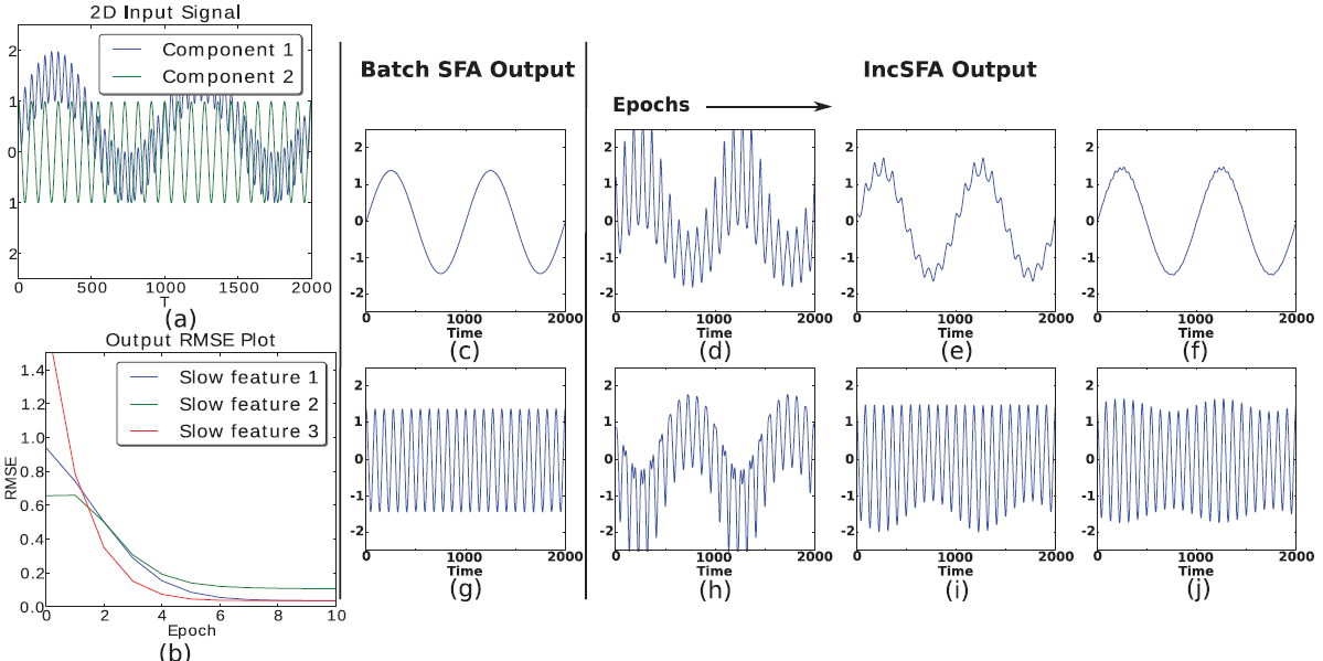
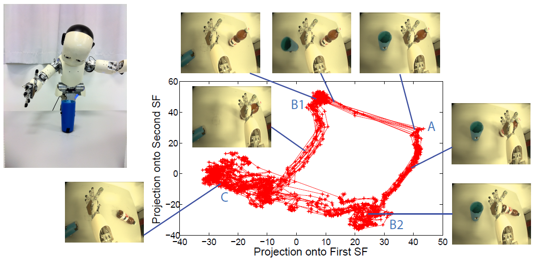
Incremental Slow Feature Analysis (IncSFA) is a low complexity, unsupervised learning technique that updates slow features incrementally without computing covariance matrices. IncSFA follows the learning objective of the batch SFA (BSFA), which is as follows: given an I-dimensional sequential input signal ${\bf x}(t) = [x_{1}(t), ..., x_{I}(t)]^{T},$ find a set of $J$ instantaneous real-valued functions ${\bf g}(x) = [g_{1}({\bf x}), ...,g_{J}({\bf x})]^{T},$ which together generate a $J$-dimensional output signal ${\bf y}(t) = [y_{1}(t), ...,y_{J}(t)]^{T}$ with $y_{j}(t) = g_{j}({\bf x}(t))$, such that for each $j \in \{1, ...,J\}$ $$ \Delta_{j} = \Delta(y_{j}) = \langle\dot{y}_{j}^{2}\rangle \quad \text{is minimal} $$ under the constraints $$ \langle y_{j} \rangle = 0\quad\textrm{(zero mean),}$$ $$ \langle y_{j}^{2} \rangle = 1\quad\textrm{(unit variance),} $$ $$ \forall i < j: \langle y_{i}y_{j} \rangle = 0\quad\textrm{(decorrelation and order),}$$ where $\langle \cdot \rangle$ and $\dot{y}$ indicates temporal averaging and the derivative of $y$, respectively. The problem is to find instantaneous functions $g_j$ that generate different output signals varying as slowly as possible. These functions are called slow features. See Figure 1 for a visual example of the meaning of a slow feature. The constraints together avoid a trivial constant output solution. The decorrelation constraint ensures that different functions $g_j$ do not code for the same features.

BSFA solves a linear approximation of the above problem through a simpler eigenvector approach. It applies batch Principle Component Analysis (PCA) twice. The first PCA is used to normalize the input ${\bf x}$ to have a zero mean and identity covariance matrix (whitening). The second PCA is applied on the derivative of the normalized input $\dot{{\bf z}}$. The eigenvectors with the least eigenvalues are the slow feature vectors.

IncSFA replaces the batch PCA algorithms with their incremental alternatives. To replace the first PCA, IncSFA uses the state-of-the-art Candid Covariance-Free Incremental PCA (CCIPCA). CCIPCA incrementally whitens the date without keeping an estimate of the covariance matrix. Except for the low-dimensional derivative signals $\dot{{\bf z}}$, CCIPCA cannot replace the second PCA step. It takes a long time to converge to the slow features, since they correspond to the least significant components. Minor Components Analysis (MCA) incrementally extracts principal components, but with a reversed preference: it extracts the components with the smallest eigenvalues fastest. IncSFA uses a modified version of Peng's low complexity MCA updating rule, and Chen's Sequential Addition technique to extract multiple slow features in parallel. A high-level formulation of IncSFA is $$(\phi(t+1), {\bf V}(t+1)) = IncSFA\left(\phi(t), {\bf V}(t), {\bf x}(t), \theta(t)\right),$$ where $\phi(t) = \left(\phi_1(t), ...,\phi_J(t)\right)$ is the matrix of existing slow feature vector estimates for $J$ slow features and ${\bf V} = \left({\bf v}_1, ..., {\bf v}_K \right)$ is the matrix of $K$ principal component vector estimates used to construct the whitening matrix. Here ${\bf x}(t) \in \mathbb{R}^I, I \in \mathbb{N}$ is the input observation and $\theta$ contains parameters about setting learning rates.

For many instances, there is no need to use IncSFA instead of BSFA. But at higher dimensionality, IncSFA becomes more and more appealing. For some problems with very high dimensionality and limited memory, IncSFA could be the only option, e.g., an autonomous robot with limited onboard hardware, which could still learn slow features from its visual stream via IncSFA. The following summarizes the advantages IncSFA has over BSFA:

it is adaptive to changing input statistics;
it has linear computational efficiency as opposed to cubic of BSFA;
it has reduced sensitivity to outliers;
it adds to the biological plausibility of BSFA.

These advantages make IncSFA suitable to use for several online learning applications. A link to the Python, Matlab, javascript (browser) implementation of the IncSFA algorithm can be found in the Software section below.

Curiosity-Driven Modular Incremental SFA (Curious Dr. MISFA)

Learns the next easiest yet unknown SFA-regularity among the inputs, with theoretical guarantees!

Figure 4: Architecture of Curious Dr.\ MISFA includes (a) a reinforcement learning agent that generates an observation stream selection policy based on the intrinsic rewards, (b) an adaptive Incremental SFA coupled with Robust Online Clustering module that updates an abstraction based on the incoming observations, and (c) a gating system that prevents encoding observations that have been previously encoded.

Figure 5: Learning Problem. Given a set of time-varying observation streams, an abstraction corresponding to the easiest-encodable yet unknown observation stream is learned first. (Left-Figure) An example result after the first abstraction was learned. (Right-Figure) $\Omega ({\bf x})$ denotes the curiosity-function that maps an observation stream ${\bf x}$ to a scalar value in $[0,1]$. Difficult-to-encode observation streams have higher $\Omega$ values. Figure shows the desired result, which is a sequence of abstractions $\{\phi_i\}_{i \in \mathbb{N}}$ learned in the order of increasing $\Omega$-values of the observation streams that they encode. However, $\Omega$ is not known a priori, therefore, the learning process involves estimating both the abstractions and the $\Omega$-values. The curved arrow indicates the temporal evolution of the learning process.

Figure 6: See text for details.

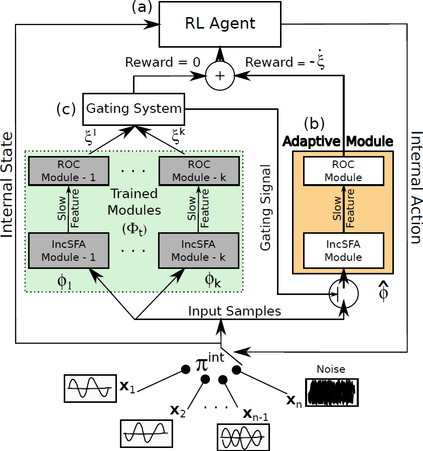
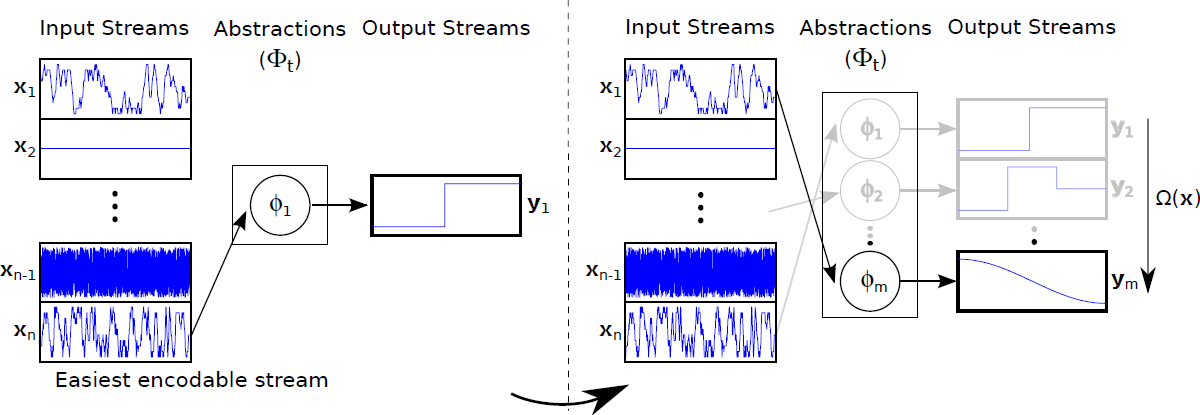
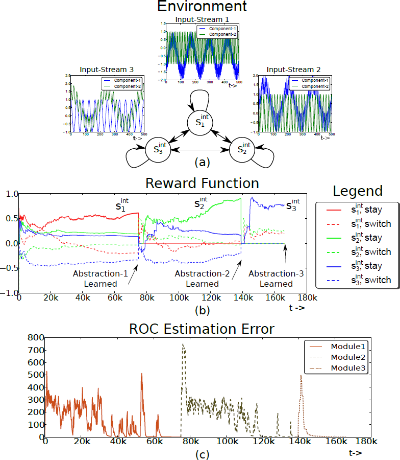
IncSFA extracts slow features without storing or estimating computationally expensive covariance matrices of the input data. This makes it suitable to use IncSFA for applications with high-dimensional images as inputs. However, if the statistics of the inputs change over time, like most online-learning approaches, IncSFA gradually forgets previously learned representations, Curiosity-Driven Modular Incremental Slow Feature Analysis (Curious Dr. MISFA) uses the theory of artificial curiosity to address the forgetting problem faced by IncSFA, by retaining what was previously learned in the form of expert modules. From a set of input video streams, Curious Dr. MISFA actively learns multiple expert modules comprising slow feature abstractions in the order of increasing learning difficulty, with theoretical guarantees.

Figure 4 shows the architecture of Curious Dr. MISFA.

Input: A set of pre-defined high-dimensional observation streams $X = \{{\bf x_1}, ..., {\bf x_n}: {\bf x_i}(t) \in \mathbb{R}^{I}, I \in \mathbb{N}\}$.
RL agent: An rl agent is in an internal environment with a state-space: $ \mathcal{S}^{\text{int}} = \{s^{\text{int}}_1,...,s^{\text{int}}_n\}$, equal to the number of observation streams. At each state the agent can take two internal actions: $\mathcal{A}^{\text{int}} = \{\text{stay}, \text{switch}\}$. The action stay makes the agent's internal state to be the same as the previous state, while switch randomly shifts the agent's state to one of the other internal states. The agent at each state $s^{\text{int}}_i$ receives a fixed $\tau$ time step sequence of observations (${\bf x}$) of the corresponding stream ${\bf x}_i$.
Adaptive IncSFA-ROC module An adaptive IncSFA is coupled with a Robust Online Clustering (ROC) algorithm to learn an abstraction $\widehat{\phi}$ based on the incoming observations. $\xi$ denotes the estimation-error made by the IncSFA-ROC for the input-samples ${\bf x}$.
Gating system The gating system contains previously learned frozen abstractions $\{ \phi_1, ..., \phi_k\}$. It prevents encoding new observations that have been previously encoded.
Goal The desired result of Curious Dr. MISFA is a sequence of abstractions $\Phi_t = \{\phi_1,...,\phi_m; m \le n\}$ learned in the order of increasing learning difficulty. Each abstraction $\phi_i: {\bf x} \rightarrow {\bf y}$ is unique and maps one or more observation streams ${\bf x} \in X$ to a low-dimensional output ${\bf y}(t) \in \mathbb{R}^J, J \in \mathbb{N}$. However, since the learning difficulty of the observation streams is not known a priori, the learning process involves estimating not just the abstractions, but also the order in which the observation streams are encoded. To this end, Curious Dr. MISFA uses the internal RL agent to learn an optimal observation stream selection policy $\pi^{\text{int}}: \mathcal{S}^{\text{int}} \rightarrow \mathcal{A}^{\text{int}}$ that optimizes the following cost-function: $$ \mathcal{J} = \min_{\pi^{\text{int}}} ~ (\langle\dot{\xi}\rangle_t^{\tau}, \langle\xi\rangle_t^{\tau}).$$ The above equation is a Multi-Objective Reinforcement Learning problem, where $\langle\dot{\xi}\rangle_t^{\tau}$ is time-derivative of the $\tau$-window averaged error $\langle\xi\rangle_t^{\tau}$. Minimization of the first objective would result in a policy that will shift the agent to states where the error decreases sharply ($\langle\dot{\xi}\rangle_t^{\tau} < 0 $), indicating faster learning progress of the abstraction-estimator. Minimization of the second objective results in a policy that improves the developing abstraction to better encode the observations. The two objectives are correlated but partially conflicting. I use an approach to find a dynamically changing pareto-optimal policy, by prioritizing each objective based on the error $\xi$. To this end, the cost is scalarized in terms of a scalar reward $r^{\text{int}}$ that evaluates the input ${\bf x}$ received for the tuple $(s^{\text{int}},a^{\text{int}},s^{\text{int}}_{-})$ as follows: $$ r^{\text{int}} = \left(\alpha\langle\dot{\xi}\rangle_t^{\tau} + \beta Z(|\delta- \langle\xi\rangle_t^{\tau}|)\right),$$ where $Z$ is a normally distributed random variable with mean $\delta$ and standard deviation $\sigma$. Here, $\alpha,~\beta,~\delta$ and $\sigma$ are constant scalars.
Exploration-Exploitation Tradeoff To balance between exploration and exploitation, a decaying $\epsilon$-greedy strategy over the policy $\pi^{\text{int}}$ is used to carry out an action (stay or switch) for the next iteration. When the $\epsilon$ value decays to zero, the agent exploits the policy and an abstraction is learned.

Figure 6 shows a simple proof-of-concept experimental result conducted using three 2D oscillatory audio streams. The environment has three internal states $\mathcal{S}^{\text{int}} = \{s^{\text{int}}_1, s^{\text{int}}_2, s^{\text{int}}_3\}$ associated with the observation streams (Figure 6(a)). The stream ${\bf x}_1$ is the easiest signal to encode followed by the input streams ${\bf x}_2$ and ${\bf x}_3$. The dynamics of the algorithm can be observed by studying the time varying reward function $R^{\text{int}}$ and the ROC estimation error $\xi$. Figure 6(b) shows the reward function for a single run of the experiment. Solid lines represent the reward for the action stay in each state $s^{\text{int}}_i$, while the dotted lines represent the marginalized reward for the action switch at each state. For the sake of explanation, the learning process can be thought of as passing through three phases, where each phase corresponds to learning a single abstraction module.
Phase 1: At the beginning of Phase 1, the agent starts exploring by executing either stay or switch at each state. After a few hundred algorithm iterations, the reward function begins to stabilize and is such that $R^{\text{int}}(s^{\text{int}}_1,$ stay$) > R^{\text{int}}(s^{\text{int}}_2,$ stay$) > R^{\text{int}}(s^{\text{int}}_3,$ stay$) > 0$, ordered according to the learning difficulty of the observation streams. However, the reward components for the switch action are either close to zero or negative. Therefore, the policy $\pi^{\text{int}}$ converges to the optimal policy (i.e. to stay at the state corresponding to the easiest observation stream ${\bf x}_1$ and switch at every other state). As $\epsilon$ decays, the agent begins to exploit the learned policy, and the adaptive IncSFA-ROC abstraction $\widehat{\phi}$ converges to the slow feature corresponding to the observation stream ${\bf x}_1$. The ROC estimation error (Figure 6(c)) decreases and falls below the threshold $\delta$, at which point, the abstraction is added to the abstraction set $\Phi$. The increase in the reward value of $R^{\text{int}}(s^{\text{int}}_1,$ stay$)$ near the end of the phase is caused by the second term ($\sum_{\tau}\left(Z(|\delta - \xi^{roc}|\right)$) in the reward equation. Both $\epsilon$ and $R^{\text{int}}$ are reset and the algorithm enters Phase 2 at ($t \approx 75k$).
Phase 2: The agent begins to explore again, however, it does not receive any reward for the ($s^{\text{int}}_1$, stay) tuple because of the gating system. After a few hundred algorithm iterations, $R^{\text{int}}(s^{\text{int}}_2,$ stay$) > R^{\text{int}}(s^{\text{int}}_3,$ stay$) > R^{\text{int}}(s^{\text{int}}_1,$ stay$)=0$, the adaptive abstraction converges, but to the slow feature corresponding to the observation stream ${\bf x}_2$.
Phase 3: The process continues again until the third abstraction is learned. A link to the Python implementation of the Curious Dr. MISFA algorithm can be found in the Software section below.

Continual Curiosity-Driven Skill Acquisition (CCSA)

An obsessed lifelong skill learner from raw-pixel vision.

Figure 7: High-level control flow of the Continual Curiosity-Driven Skill Acquisition (CCSA) framework. (a) The agent starts with a set of pre-defined or previously acquired exploratory behaviors (represented as exploratory options). (b) It makes high-dimensional observations upon actively executing the exploratory options. (c) Using the Curious Dr.\ MISFA algorithm, the agent learns a slow feature abstraction that encodes the easiest to learn yet unknown regularity in the input observation streams. (d) The slow feature abstraction outputs are clustered to create feature states that are augmented to the agent's abstracted state space. (e) A Markovian transition model of the new abstracted state space and an intrinsic reward function are learned through exploration. (f) A deterministic policy is then learned via model-based Least Squares Policy Iteration (Model-LSPI) and a target option is constructed. The deterministic target-option's policy is modified to a stochastic policy in the agent's new abstracted states and is added to the set of exploratory options.

Figure 8: Reuse of the learned target options. For each target option learned (represented by pink dotted box), two new exploratory options (Biased Initialization and Explore and Policy Chunk and Explore) are added to the input exploratory-option (represented by red dashed boxes) set. Biased Initialization and Explore option biases the agent to explore first the state-action tuples where it had previously received maximum intrinsic rewards, while the Policy Chunk and Explore option executes the deterministic target-option's policy before exploration.

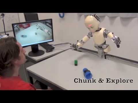
Click to open the YouTube video.

Video: This video demonstrates how CCSA enables an iCub humanoid robot to incrementally acquire skills in order of increasing learning difficulty, from its onboard high-dimensional camera inputs and low-level kinematic joint maps, driven purely by its intrinsic motivation. The video has three parts. The first part shows how the iCub finds it interesting to topple the cup placed on the table. It learns a topple skill eventually. In the second part, the robot continues to explore by reusing the topple skill and discovers that it is able to grasp the cup. It eventually acquires a skill to succesfully grasp the cup. In the third part, the iCub locates an external reward present for placing the cup at a desired location.

Curious Dr. MISFA algorithm actively learns multiple slow feature abstractions in the order from least to most costly, as predicted by the theory of artificial curiosity. Each abstraction learned encodes some previously unknown regularity in the input observations, which forms a basis for acquiring new skills. Continual Curiosity-Driven Skill Acquisition (CCSA) framework translates the abstraction learning problem of Curious Dr. MISFA to a continual skill acquisition problem. Using CCSA, a humanoid robot driven purely by its intrinsic motivation can continually acquire a repertoire of skills that map the many raw-pixels of image streams to action-sequences.

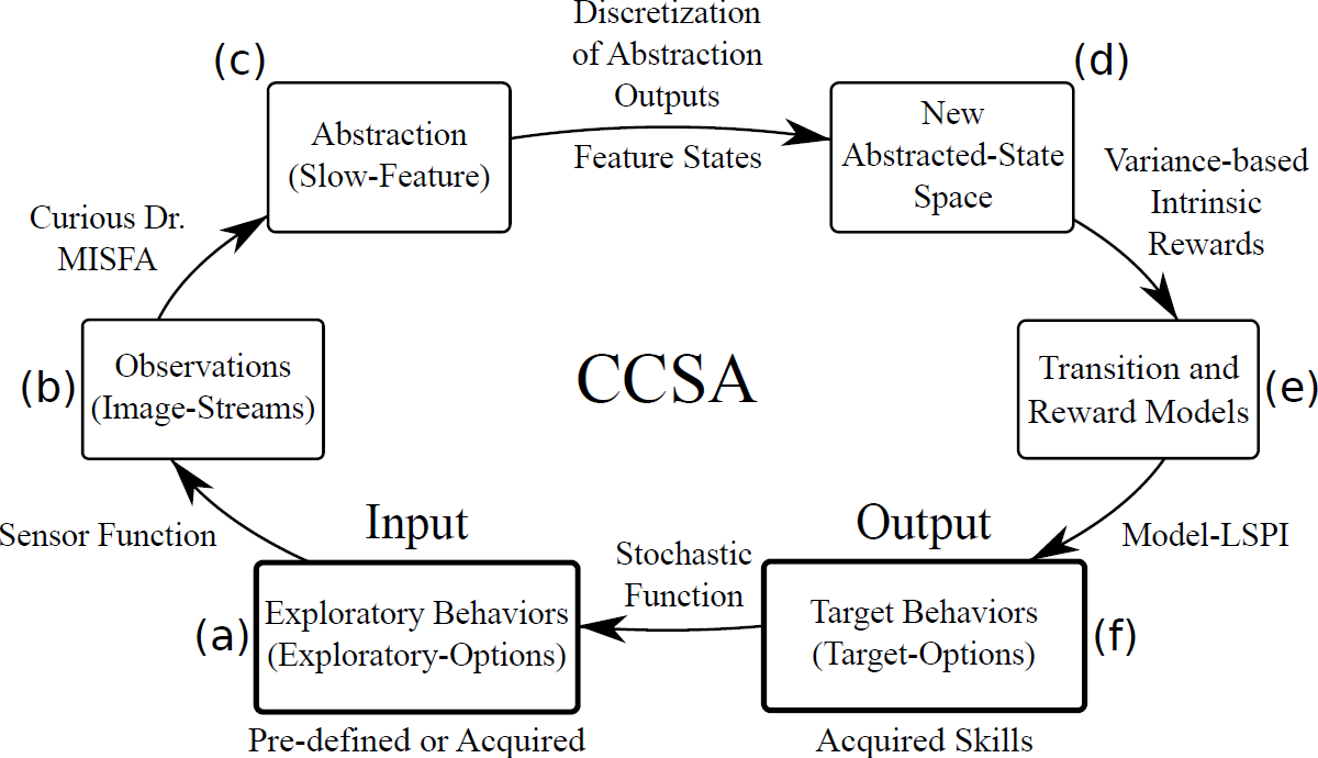
Figure 7 illustrates the overall CCSA framework. The learning problem associated with CCSA can be described as follows. From a set of pre-defined or previously acquired input exploratory behaviors that generate potentially high-dimensional time-varying observation streams, the objective of the agent is to (a) acquire an easily learnable yet unknown target behavior and (b) re-use the target behavior to acquire more complex target behaviors. The target behaviors represent the skills acquired by the agent. A sample run of the CCSA framework to acquire a skill:

The agent starts with a set of pre-defined or previously acquired exploratory behaviors. I make use of the options framework to formally represent the exploratory behaviors as exploratory options. Each exploratory option is defined as a tuple $\langle \mathcal{I}^e_i, \beta^e_i, \pi^e_i \rangle$, where $\mathcal{I}^e_i$ is the initiation set comprising states where the option is available, $\beta^e_i$ is the option termination condition, which will determine where the option terminates (e.g., some probability in each state), and $\pi^e_i$ is a pre-defined stochastic policy.
The simplest exploratory option policy is a random walk. However, I use a more sophisticated variant uses a form of initial artificial curiosity, derived from error-based rewards. This exploratory-option's policy $\pi^e$ is determined by the predictability of the observations ${\bf x}(t)$, but can also switch to a random walk when the environment is too unpredictable.
The agent makes high-dimensional observations through a sensor-function, such as a camera, upon actively executing the exploratory options.
Using the Curious Dr. MISFA algorithm, the agent learns a slow feature abstraction that encodes the easiest to learn yet unknown regularity in the input observation streams.
The slow feature abstraction outputs are clustered to create feature states that are augmented to the agent's abstracted state space, which contains previously encoded feature states.
A Markovian transition model is learned by exploring the new abstracted state space. The reward function is also learned through exploration, with the agent being intrinsically rewarded for making state transitions that produce a large variation (high statistical variance) in slow feature outputs. This specialized reward function is used to learn action-sequences (policy) that drives the agent to states where such transitions will occur.
Once the transition and reward functions are learned, a deterministic policy is learned via model-based Least-Squares Policy Iteration . The learned policy and the learned slow feature abstraction together constitute a target option, which represents the acquired skill.

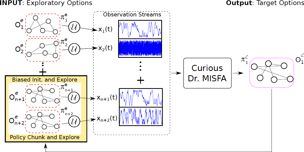
The deterministic target-option's policy is modified to a stochastic policy in the agent's new abstracted states. This is done by constructing two new exploratory options that are based on the target option that was learned last. The first option, called the biased initialization and explore, biases the agent to explore first the state-action tuples where it had previously received maximum intrinsic rewards. Whereas the second option, called the policy chunk and explore, executes the deterministic target-option's policy before exploration. For each target option learned, these two exploratory options are added to the input exploratory-option set (Figure 8). In this way, the agent continues the process of curiosity-based skill acquisition by exploring among the new exploratory option set to discover unknown regularities. A complex skill can be learned as a consequence of chaining multiple skills that were learned earlier.

CCSA is a task-independent algorithm, i.e., it does not require any design modifications when the environment is changed. However, CCSA makes the following assumptions: (a) The agent's default abstracted state space contains low-level kinematic joint poses of the robot learned offline using Task Relevant Roadmaps. This is done to limit the iCub's exploration of its arm to a plane parallel to the table. This assumption can be relaxed resulting in a larger space of arm exploration of the iCub, and the skills thus developed may be different. (b) CCSA requires at least one input exploratory option. To minimize human inputs into the system, in the experiments at $t=0$, the agent starts with only a single input exploratory option, which is a random-walk in the default abstracted state space. However, environment or domain specific information can be used to design several input exploratory options in order to shape the resulting skills. For example, random-walk policies mapped to different sub-regions in the robot's joint space can be used.

Software

Python and Matlab codes of the above algorithms can be found here .

References

V. R. Kompella. Slowness Learning for Curiosity-driven Agents, Ph.D. Thesis, 2014.
Link to manuscript.
V. R. Kompella, M. Luciw and J. Schmidhuber. Incremental Slow Feature Analysis, 22^nd International Joint Conference on Artificial Intelligence (IJCAI), Barcelona, 2011.
Link to paper.
V. R. Kompella, M. Luciw and J. Schmidhuber. Incremental Slow Feature Analysis: Adaptive Low-Complexity Slow Feature Updating from High-Dimensional Input Streams, Neural Computation Journal, Vol. 24 (11), pp. 2994--3024, 2012.
Link to preprint.
V. R. Kompella, L. Pape, J. Masci, M. Frank and J. Schmidhuber. "AutoIncSFA and Vision-based Developmental Learning for Humanoid Robots, 11^th IEEE-RAS International Conference on Humanoid Robots (Humanoids), Bled, Slovenia, 2011.
Link to paper. Link to Video.
M. Luciw, V. R. Kompella and J. Schmidhuber. Hierarchical Incremental Slow Feature Analysis , Workshop on Deep Hierarchies in Vision (DHV, Vienna), 2012.
Link to poster.
V. R. Kompella, M. Luciw, M. Stollenga, L. Pape and J. Schmidhuber. Autonomous Learning of Abstractions using Curiosity-Driven Modular Incremental Slow Feature Analysis. (Curious Dr. MISFA) , IEEE International Conference on Developmental and Learning and Epigenetic Robotics (ICDL-EpiRob), San Diego, 2012.
Link to paper. Link to Video.
M. Luciw*, V. R. Kompella*, S. Kazerounian and J. Schmidhuber. An intrinsic value system for developing multiple invariant representations with incremental slowness learning, Frontiers in Neurorobotics, Vol. 7 (9), 2013. *Joint first authors.
Link to paper.
V. R. Kompella, M. Stollenga, M. Luciw and J. Schmidhuber. Explore to See, Learn to Perceive, Get the Actions for Free: SKILLABILITY, Proc. of IEEE International Joint Conference on Neural Networks (IJCNN), Beijing, 2014.
Link to paper.